Classifier-free guidance
What CFG actually does
Classifier-free guidance is switched on in almost every diffusion and flow sampler. It improves prompt adherence and usually quality — but what it does to the output distribution is still disputed. An idealised model, measured against a real 3D generator.
Classifier-free guidance (CFG)[1] is simple to state. At every sampling step, run the model twice — once with the condition, once without — and combine the two outputs with a coefficient γ. A larger γ gives outputs that follow the condition more closely and, in practice, look better. This is reliable enough that almost nobody samples at γ=1.
The earliest explanation of why is that CFG lowers the sampling temperature: the distribution gets sharper and concentrates on high-probability regions. That account is everywhere, including most tutorials.
It is probably wrong. Over the past two years several papers have each rejected the others’ picture of CFG, and the disagreement is not about wording — it is about what CFG does to the output distribution.
Above all of that sits a contradiction that everyone assumes away:
If CFG pushes the distribution away from the real data, why is γ=5 better than γ=1?
This article answers in three layers.
First, what CFG is trying to do (Section 2). Under an idealised model — CFG applied once, and the sampler returning exactly the distribution that one application defines — what happens as γ grows: which modes become more common, where each mode’s centre moves, and how much variation is left within a mode. All three have closed forms.
Second, where reality departs from the ideal (Sections 3–4). The sampled distribution is not the idealised one, for two reasons: the tilt and the noising happen in the wrong order, and CFG is applied not once but at every step. The first reason has nothing to do with step count or with whether the sampler is deterministic — infinitely many steps would not remove it.
Third, why quality improves anyway (Sections 5–6). Because CFG is not correcting the distribution. It is correcting the model’s error.
Section 1 fixes the formula and notation. The exposition uses rectified flow / flow matching; DDPM and DDIM appear only for comparison.
01The formula, and the distribution behind it
Start with the sampler. Rectified flow begins at pure noise and follows a trajectory to clean data: at each step the model takes the current x and the noise level t and returns a velocity — which way to move, and how far. Integrating those steps to t=0 gives a sample.
Without CFG the model runs once per step: it sees the condition, returns v_c, and the sampler steps along v_c.
CFG changes exactly this step. The model runs twice — once with the condition, giving v_c, once with the condition removed, giving v_u — and the sampler steps along a linear combination of the two:
step taken = v_u + γ · (v_c − v_u)γ is the guidance_scale of every pipeline. At γ=1 the right-hand side collapses to v_c and CFG is off; at γ>1 the sampler continues a little further along the difference the condition made.
DDPM and DDIM predict noise ε rather than velocity, but the CFG formula is identical with ε in place of v. Everything below holds in both parameterisations; the reason is in the collapsible box.
What this step does to the distribution
Velocity and score (∇log p) determine each other — given one you can compute the other. So a linear combination of two velocities is a linear combination of two scores:
(1−γ) · ∇log p(x) + γ · ∇log p(x|c)and that is the gradient of log[ p(x|c)^γ · p(x)^(1−γ) ]. Each CFG step follows the score of that distribution. Rearranged:
p_γ(x|c) ∝ p(x|c) · r(x)^(γ−1) where r(x) = p(x|c) / p(x)So at the level of distributions, γ reweights p(x|c) by r: regions where r is large are amplified, regions where r is small are suppressed, and γ sets how hard.
Multiplying a distribution by a weight function and renormalising has a name: a tilt. Throughout, “tilt” means this operation — CFG is a tilt of p(x|c) with weight r^(γ−1).
Three terms recur below; definitions first:
| term | meaning |
|---|---|
| density | The relative likelihood of one specific output. Where p(x|c) is high, samples land more often. |
| share | After many samples, the fraction that fall into one category of outputs. The share is the density integrated over that category, and it is the quantity an experiment can actually count. |
| r | The density of one output under p(x|c), divided by its density under p(x). |
r is the most important quantity in this article and deserves a moment. It measures how much an output owes its existence to the condition:
rlarge — this kind of output essentially only appears when the condition is givenrnear 1 — it appears just as readily without the condition, so it says little about the condition
Equivalently, r is proportional to the probability that the condition was c given this output — the classifier implicit in the model. CFG never trains a classifier, but it steers by this ratio at every step.
Derivation: Bayes, twice
Classifier guidance multiplies the classifier term by γ: the score becomes ∇log p(x) + γ∇log p(c|x). Scaling a log-gradient by γ raises the term to the power γ, so this is the score of p(x)·p(c|x)^γ.
Bayes removes the classifier: ∇log p(c|x) = ∇log p(x|c) − ∇log p(x). Substituting gives (1−γ)∇log p(x) + γ∇log p(x|c) — the CFG combination — whose distribution p(x|c)^γ p(x)^(1−γ) rearranges to the form above.
Flow-matching conversion: ∇log p_t(x) = −[x + (1−t)v(x,t)]/t, hence ∇log r = −((1−t)/t)(v_c − v_u). The coefficient is positive and independent of x, so every statement below about sign, zeros and monotonicity holds identically in the v and ε parameterisations.
Notation
| symbol | meaning | typical values |
|---|---|---|
| x | a data point (the model’s latent) | — |
| c | the condition | — |
| t | noise level | 0 = clean, 1 = pure noise |
| γ | guidance scale | 1 = no CFG; 5–9 in text-to-image; 100 in SDS |
| v_c, v_u | output of the conditional / unconditional branch | — |
| Δ | v_c − v_u, the direction CFG pushes | — |
| r | conditional density / unconditional density | — |
| x* | the point where Δ = 0: both branches make the same prediction | — |
02The single-step ideal: what CFG is trying to do
This section works with an idealised model that assumes two things:
- CFG is applied once, to the distribution of clean data
- The sample is drawn from the
p_γthat one application defines
Neither holds in real sampling; the next two sections take them in turn. The ideal is still worth working through: the three conclusions below survive real sampling in direction, though not in magnitude — and without the ideal there would be nothing specific to measure.
Under the ideal, raising γ does three things:
| what happens | form | |
|---|---|---|
| Effect 1: modes are reweighted | some modes are amplified and others suppressed, exponentially | share ratio ∝ (r_A/r_B)^(γ−1) |
| Effect 2: centres move, then stop | each mode’s centre leaves its original position but stops at a fixed point | stops at x* |
| Effect 3: each mode narrows | samples within one mode become more alike | variance ∝ 1/(γ−1) |
1 = no CFG. Text-to-image typically uses 5–9.
Width of the unconditional distribution. Each mode is fixed at 0.5.
Effect 1Modes are reweighted by r
Why this holds: p_γ is p(x|c) times r^(γ−1). A single mode is narrow, so r is approximately a constant r_j across it, and the mode’s share is simply its original share times r_j^(γ−1):
share_j ≈ w_j · r_j^(γ−1) w_j = share of mode j under p(x|c) share_A / share_B = (w_A / w_B) · (r_A / r_B)^(γ−1)γ sits in the exponent, so the gap opens exponentially. But the point is not the exponent. It is that the quantity being amplified is the ratio of r, not the ratio of densities. In the figure, mode A starts at share 0.6 and B at 0.4 — but A sits at the centre of the unconditional distribution (dashed) and B in its tail, so r_B > r_A. Raise γ to 4 and the taller peak sinks while the shorter one rises, crossing at γ≈1.8.
CFG does not pick the most probable mode. It picks the mode that is best explained only by the condition.
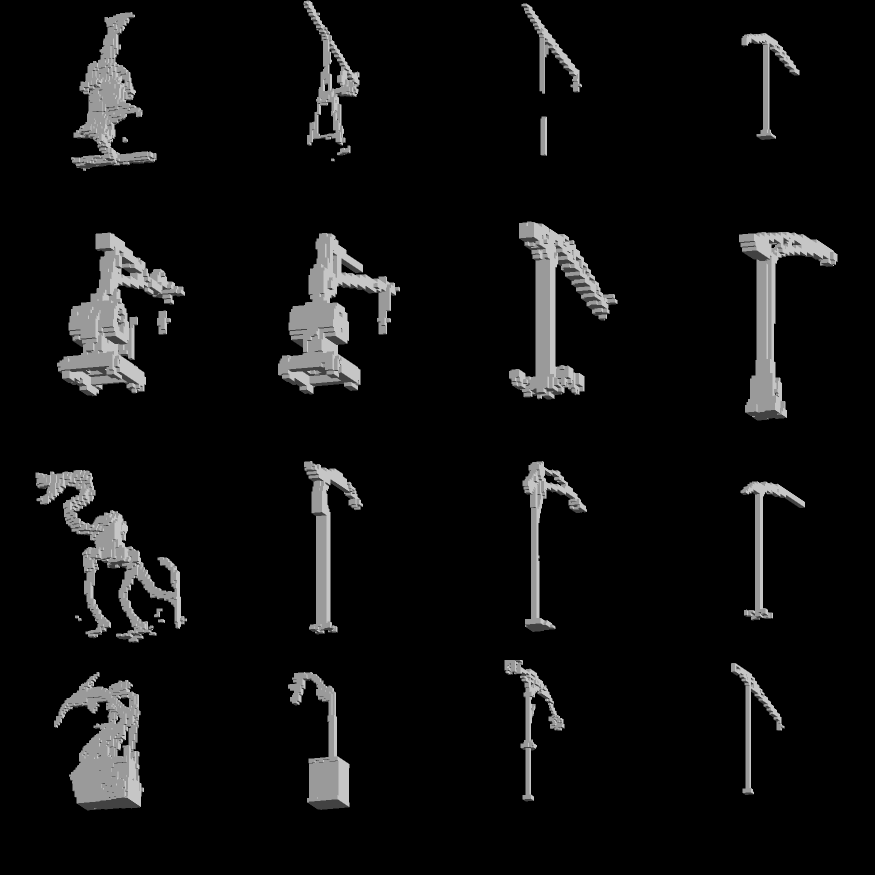
a crane; rows are seeds, columns are γ, and within a row only γ changes. At γ=1 the column is creatures with legs and bodies; by γ=6 every one is a tower crane. The English word names both the machine and the bird, and without CFG the model produces both; as γ grows, the bird reading disappears.The seeds were not hand-picked: the 16 seeds were scored on the mode axis at γ=1 and the four most creature-like were taken.
a crane, and at γ=1 the tower is the minority at 10%; as γ grows it rises to 30%. If CFG were low-temperature sampling, the minority should be driven toward zero while the majority (birds) grows — the measurement shows the opposite. The tower is amplified because the unconditional branch already produces birds and other creatures readily: the tower is the reading that is only likely given the condition, so its r is larger.The lower line is the control: with the condition changed to
a crane, the long-legged wading bird, the same tower mode falls from 0.047 to 0.008. The reversal shows that what gets amplified is not the tower mode as such, but whatever the condition makes r large for.Why a popular account fails: CFG is not low-temperature sampling
Low-temperature sampling draws from p(x|c)^γ — the numerator alone — and its share ratio is (w_A/w_B)^γ, which can only make the larger mode larger. CFG carries the denominator p(x)^(1−γ), which penalises precisely the outputs that are common without the condition. On the figure’s example:
low temperature: A keeps winning (0.6/0.4)^γ grows monotonically CFG: B overtakes reversal beyond γ≈1.8Same distribution, same γ, and the two operations push samples toward opposite modes. “CFG is roughly a temperature” is therefore not imprecise but wrong: on the question of which mode wins, the sign is reversed.
Effect 2Each mode’s centre moves, then stops
Within a mode, the centre moves away from the unconditional distribution — but not indefinitely. Give the difference inside the CFG bracket a name:
Δ = v_c − v_u CFG is: start from v_u, then go γ times further along Δx* is where Δ = 0 — the point at which both branches make the same prediction.
Δ is proportional to ∇log r (the conversion is in the box above), and x* is the maximum of r, where the gradient vanishes — so Δ vanishes there too, CFG switches itself off, and samples are attracted to the point. The second small panel plots mode B’s centre against γ: a fast rise, then a plateau on x*, with almost no movement between γ=5 and γ=12.
Note the counter-intuitive consequence: the larger γ, the closer samples sit to the point where CFG itself disappears. Section 4 will show that no such point exists in the model we measured.
Effect 3Each mode narrows, at rate 1/(γ−1)
The variance within a mode falls as 1/(γ−1). The standard deviation therefore falls as 1/√(γ−1), more slowly than the centre settles — so beyond a certain γ, the samples stop changing and only become more alike.
Derivation: why 1/(γ−1)
Write β = γ−1. The target is p(x|c)·r^β; take logs and expand about x*. The first-order term of log r vanishes (it is an extremum) and the second-order term carries β, so β sets the curvature. Completing the square gives a Gaussian with covariance H⁻¹/β, where H = −∇²log r(x*). Hence the variance is proportional to 1/(γ−1), and the mean approaches x* at the same rate.
Checked numerically on the one-dimensional Gaussian example: at γ=100 the exact variance is 0.01329 and the approximation gives 0.01347.

1/(γ−1): γ−1 spans a factor of 96 and the variance only falls to 30–61%. Section 4 explains why.Drag the second slider, σu, until the unconditional distribution is as wide as a single mode (0.5): the narrowing vanishes. In other words:
Whether a mode narrows depends on how narrow the mode is relative to how wide the unconditional distribution is — the larger the gap, the stronger the narrowing. γ is only an amplifier: when the two are equally wide, any γ merely moves the mode without shrinking it.
That premise does not always hold in a real model: half of the directions violate it. Take the latent distribution under one condition, run PCA, keep the twelve leading directions, and compare conditional and unconditional widths direction by direction:
| direction | width at γ=25, relative to γ=1 |
|---|---|
| six directions where the conditional was narrower | 0.21–0.45 (narrowing, as effect 3 predicts) |
| six directions where the conditional was wider | expansion, peaking at 1.95× at γ=3 in the widest direction |
And the expansion peaks at γ=2–5 — the range people actually use. So:
CFG is not an isotropic contraction. It compresses the directions in which the conditional was already narrower and expands the ones in which it was wider. A scalar variance sums the two, shows a net contraction, and hides the fact that the two families of directions move in opposite senses.
Where samples concentrate as γ → ∞
r^(γ−1) is an exponential amplifier: in the limit, all of the mass collapses onto the point where r is largest — not the point where p(x|c) is largest.
The limit is “the c that is most distinguishable from unconditional”, not “the most typical c”. At moderate γ the two barely differ; at large γ they separate quickly.
03Where the gap between ideal and real comes from
The sampled distribution does not match the ideal p_γ, and the reason is specific: the tilt and the noising happen in the wrong order.
In the ideal model, the tilt acts on the clean-data distribution and produces p_γ. For the sampler to actually end at p_γ, what it sees at every step must be p_γ after noising — tilt first, then noise.
But what the model learned is p_t(x|c) and p_t(x): clean data noised directly, with no tilt in between. CFG can only tilt those two already-noised distributions — noise first, then tilt.
needed: clean data ──tilt──▶ p_γ ──noise──▶ what the sampler sees CFG gives: clean data ──noise──▶ two distributions ──tilt──▶ what the sampler seesThe two operations do not commute. Only with no noise at all do the two paths agree. p_γ is defined at zero noise, so p_γ itself is not miscalculated; the sampler simply follows the other path and lands somewhere else. This is not a precision issue — with infinitely many steps, a perfectly trained model and a deterministic sampler, the path is still the other one, and the result is still not p_γ.
0 = clean data, 3 ≈ pure noise. Sampling runs from right to left.
At γ=1 the two paths coincide exactly.
γμ₁+(1−γ)μ₀: the more noise, the closer CFG's path gets to this naive extrapolation, while the mean of the needed path does not move at all. Example: p₀(·|c)=N(1,1), p₀=N(0,4).04Many steps: how the three effects change
The ideal applies CFG once. Real sampling applies it at every one of several dozen steps, each at a different noise level. The same tilt does different things at different noise levels.
Prediction: each effect has its own noise window
One quantity governs all three effects: how narrow a conditional mode is against how wide the unconditional distribution is. Noise widens both, so the gap changes with the noise level — and each effect gets its own active window.
| high noise start of sampling | mid | low noise end of sampling | |
|---|---|---|---|
| Effect 1: modes reweighted | modes still merged; nothing to amplify or suppress | active | already decided; cannot change |
| Effect 2: centres move, then stop | keeps moving outward | displacement starts to converge | already resting on x* |
| Effect 3: each mode narrows | almost none — noise has flattened both widths | starts to appear | strongest |
Drag to watch the two peaks merge and the valley between them fill in.
γ scales the three curves but does not move them.
The separation sets where the middle window falls.
exp(−valley depth), borrowed from the Kramers escape rate — an approximation.Measured: one prediction out of three holds
Every measurement is on our own 3D rectified-flow model. The CFG and no-CFG arms use the same seeds and the same initial noise, and the two arms’ estimates of the clean sample are compared step by step. t′ is the noise level the model actually receives, 1 being pure noise; sampling runs from right to left over 45 steps.
| effect | predicted | measured |
|---|---|---|
| Effect 1 | strongest mid-way | Wrong. Finished within the high-noise band |
| Effect 2 | strongest at high noise | Right. Displacement peaks at the highest noise, then decays monotonically to one seventh |
| Effect 3 | strongest at low noise | Needs correction. At high noise CFG first expands the distribution; net narrowing appears only at low noise, where effect 3 is the only effect still active |
Effect 1 | Reweighting between modes: finished in the high-noise band
At every step, both arms are projected onto a mode axis and the mass on each mode is read off. The fit allows the whole cloud to translate along the axis, so what is read is mass genuinely moving from one mode to the other, not an artefact of translation.
noise level t′ | 0.992 step 1 | 0.881 | 0.832 | 0.706 |
|---|---|---|---|---|
| fraction of the between-arm weight gap completed | 61% | 87% | 98% | 100% |
The second row is how much of the eventual difference in mode weight between the two arms has already appeared by that noise level. 61% in the first step, 98% by t′=0.832, nothing further below t′=0.71. The prediction said mid-way; the measurement says it is essentially over at the highest noise.
This contradicts the prediction head-on: at t′=0.99 the two modes overlap completely — how can mass move between them? Because noising does not change mixture weights. The forward process shrinks each component toward the origin and blurs them into one another, but the weight in front of each component is untouched at every noise level. What high noise destroys is the components’ positions — which is why a single sample cannot be classified there — not the weight that CFG acts on.
Separating the two arms shows one more thing: the CFG arm’s mode weight stops changing at t′=0.96 and moves by 0.002 over the remaining 39 steps, while the no-CFG arm keeps redistributing until t′≈0.71. The gap keeps widening because the no-CFG arm is moving — not because CFG is still acting.
Effect 2 | Centres move, then stop: the first half holds, the second does not
noise level t′ | highest | mid | end |
|---|---|---|---|
| distance between the two arms’ centres | 2.60 | 0.46 | 0.39 |
The unit is the no-CFG arm’s spread at the end. The displacement is largest at the highest noise and decays monotonically to one seventh — the “strongest at high noise” prediction holds, the only one of the three that does.
But the ideal also said the centre would stop at x*, where both branches agree. It does not. Fit a saturating curve to the displacement against γ, and the measured points overshoot the curve’s own limit — this model has no x*. Samples stop because the 45 steps run out, not because they have reached that point.
Effect 3 | Each mode narrows: expansion first, narrowing late
x₀ = x_t − t·v, with the no-CFG arm's final value set to 1. (Both arms share their initial noise, so x_t itself is identical at the first step.) At t′=0.977 the CFG arm is at 1.9× — CFG is expanding here, not narrowing. The reason: at high noise the model has seen almost no signal, so every seed's x₀ estimate under one condition is nearly the same — the no-CFG arm has almost no diversity to begin with. CFG multiplies the small seed-to-seed differences by γ−1, and at this noise level that term barely decays, so the ratio blows up.The prediction said strongest at low noise. In the high-noise band the measured direction is the reverse: CFG does not narrow the distribution there — it expands it, to 1.9× (figure above; the reason is in its caption). The expansion decays as noise falls, net narrowing appears only below t′≈0.65, and what survives to the end is 8% of the expansion (28% and 16% on two other inputs).
This explains why Section 2’s 1/(γ−1) is so far off: γ−1 spans a factor of 96 and the variance only falls to 30–61% — most of the “contraction” is undoing the earlier expansion.
Half the prediction still stands: at low noise, effect 3 is the only effect still active — not because narrowing is strongest there, but because the other two have stopped.
What survives from Section 2
Every directional conclusion holds; no numerical form matches the ideal model.
| effect | direction: holds | magnitude: fails |
|---|---|---|
| Effect 1 | Modes are selected by r, not by density. Under a crane the minority mode at 10% is amplified threefold; low temperature would drive a minority to zero | The ideal predicts share ratios growing exponentially in γ. They do at small γ; at large γ they barely move |
| Effect 2 | Centres move away from the unconditional distribution | The ideal predicts a stop at x*. The centre does not stop, and overshoots the limit of a fitted saturating curve — no x* in this model |
| Effect 3 | Variance falls with γ | The ideal predicts variance ∝ 1/(γ−1). It falls far more slowly and has a floor: γ−1 spans 96×, the variance reaches only 30–61% |
The directional statements are not merely “still looking right”; several are theorems. Wu et al.[2] prove that CFG lowers the differential entropy of the output distribution and raises classification confidence, for DDPM and DDIM alike; Li and Jiao[3] prove for general data distributions that CFG lowers the expected reciprocal of the classifier probability. The directional conclusions are the most reliable ones — and they are also the useful ones.
05So why does quality improve?
Here is the real problem. None of the three effects — reweighting, centre shift, narrowing — explains why generation quality goes up. Section 2’s last conclusion makes it worse: at large γ, samples concentrate on the point most distinguishable from the unconditional distribution, not on the most typical one. That should look less like real data.
One premise is missing:
Everything so far assumes the model is correct. Admit that the model itself is biased, and the contradiction disappears.
A very short argument
Suppose the model at γ=1 returns the true conditional distribution. Then any γ>1 can only move the result away from the truth, and every quality metric should degrade monotonically from γ=1 upward.
In practice nobody samples at γ=1. The best γ is always above 1 — universal experience, and the shape of every FID-versus-γ curve in the literature. Therefore:
some γ > 1 beats γ = 1 ⟹ the model at γ = 1 was already biasedSimple reasoning, large conclusion: CFG is not correcting the distribution. It is correcting the model’s error.
What error, and why r can fix it
Karras et al.[4] give a concrete account: score-matching training makes the model place probability where real data never occur, producing outliers, and CFG removes those outliers.
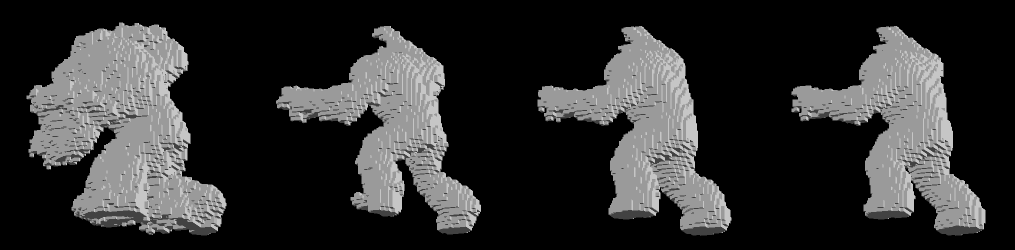
Why score matching puts probability where there is no data
The training objective minimises KL(p_data ‖ p_model), and the two ways of being wrong cost very differently:
- data present, model density near zero — the
logterm diverges; infinite penalty - data absent, model density positive — the
p_data ≈ 0factor in front makes the penalty almost nothing
Missing real data is catastrophic; spreading density where there is none is nearly free. With unlimited capacity both can be satisfied at once; with finite capacity they conflict, and the model errs toward spreading.
The learned density is therefore flatter and wider than the truth, with gaps that should be empty filled in. Karras et al.’s two-dimensional example shows exactly this: a tree-shaped distribution whose learned density is visibly wider, so samples fall into the spaces between branches.
This is an estimation error, not a property of diffusion itself — with enough data and capacity, score matching converges to the true score. Section 6’s “the CFG strength a model needs reflects its error” rests on this.
What matters is the nature of this error: it comes from the model being insufficiently accurate, not from the condition — the conditional and unconditional branches make the same kind of mistake, only more severely on the unconditional side. Because both branches have it, it cancels in the ratio r: those regions have r ≈ 1, and r^(γ−1) suppresses them.
This yields a falsifiable prediction: only the error shared by both branches is removed; error specific to the conditional branch is amplified. That is different from “CFG removes outliers”, under which it would not matter which branch the error came from.
The three effects, read again
| effect | distribution view | error view |
|---|---|---|
| Effect 1 | reweight modes by r | suppress modes that exist only because density was spread |
| Effect 2 | move toward where the branches agree | leave the regions dominated by the unconditional branch’s error |
| Effect 3 | narrow each mode | remove the excess variance that spreading added |
This agrees with the line of work that decomposes Δ into components — Li et al.[5] isolate a term that “suppresses generic features common across unconditional data”. Two descriptions of the same thing.
Where the optimum γ lies
Too small, and the error is not fully cancelled; too large, and the bias the tilt introduces exceeds the error it removes. The best γ balances the two — which is why quality metrics are U-shaped in γ.
And a part that has nothing to do with distributions
Some of the “improvement” is not distributional at all. People prefer high contrast, saturated colour and clean composition, and high γ delivers exactly those. Distribution metrics cannot see this; human evaluation can — and aesthetic preference is a different thing from “closer to real data”, sometimes the opposite.
So “looks better” is at least three things stacked together: error cancelled (a genuine improvement), bias from the tilt (a genuine degradation), and aesthetic preference (a property of the metric). Separating them is what this article set out to do.
06What this means for training
If CFG is fundamentally correcting model error, a few conclusions follow directly.
The CFG strength a model needs reflects its error
In the limit, a perfectly accurate model needs no CFG — so the more accurate the model, the smaller the γ it needs. The same fact can be exploited the other way round: Karras et al.[4] replace the unconditional branch with a deliberately under-trained version of the same model, so that r points more purely along the error direction — FID 1.01 on ImageNet. Both routes share a premise: what CFG acts on is the error, not the condition.
Two different thresholds when tuning γ
Raising γ meets two events in turn: a value where quality peaks, and, further on, visible defects — oversaturation in images, structural collapse in geometry. These are two different thresholds, set by different factors.
| set by | as the model improves | |
|---|---|---|
| the γ where quality peaks | the gap between the conditional and unconditional branches’ errors | falls |
| the γ where defects appear | the model’s own accuracy — larger γ is more extrapolation | rises |
So the usable range between them widens as training proceeds. We have not seen this separation reported, and it can be measured on any series of checkpoints. Tracking the optimal γ also shows how much the conditional branch has improved relative to the unconditional one — γ stops being merely an inference-time knob.
Designing a schedule
| band | what applying CFG here buys |
|---|---|
| high noise | Which mode a sample lands in, and where its centre moves, are both decided here. Cutting this band means giving up control of the result |
| low noise | Only effect 3 is still active. Cut this band and the narrowing is gone |
So a schedule that applies CFG only within some noise band can buy very different things on different models, depending on where that model’s modes are decided. That position is measurable — apply CFG band by band and compare mode shares — so measure it before choosing a schedule.
How the experiments were run
Scope: every measurement is on one model — an image/text-conditioned 3D rectified-flow model producing a 64³ occupancy field. The results describe what happens on that model; they do not vouch for others.
| Model | image/text-conditioned 3D rectified flow, 45 steps, 64³ continuous occupancy output |
| Scale | ≈13,000 samples; ≈5 GPU-hours on 8×B200 |
| γ grid | 1, 1.25, 1.5, 2, 3, 5, 6, 9, 15, 25; 128 seeds per point |
| Pairing | the CFG and no-CFG arms share seeds and initial noise, so per-sample comparison is valid |
| Variance | mean pairwise squared distance over 2 (the trace of the covariance); standard error from 400 bootstrap resamples |
| Mode classification | occupancy pooled to 16³ and normalised by total mass; one axis built from hand-picked exemplars; leave-one-out accuracy 93.3% |
| Rendering | DDA with flat per-face shading, normals from the cube face the ray crosses. Not a smooth isosurface — the data are voxels |
Implementation details that mattered: γ=1 takes a different code path (the pipeline branches on cfg>1); the “unconditional” branch ships with a default negative prompt, not an empty string; Euclidean distance in latent space barely separates conditions (total variance differs by only 12% across nine conditions), so all clustering is on geometric features; noise bands must be defined by the t′ the denoiser actually receives, not by step index; and the sampler is chaotic — any perturbation diverges to 0.08–0.11σ over 45 steps, so the t′<0.6 row is only 1.7× that floor and only t′<0.8 is unambiguous.
References
- Jonathan Ho, Tim Salimans. Classifier-Free Diffusion Guidance. NeurIPS 2021 Workshop on Deep Generative Models. arXiv:2207.12598
- Yuchen Wu, Minshuo Chen, Zihao Li, Mengdi Wang, Yuting Wei. Theoretical Insights for Diffusion Guidance: A Case Study for Gaussian Mixture Models. ICML 2024. arXiv:2403.01639
- Gen Li, Yuchen Jiao. Provable Efficiency of Guidance in Diffusion Models for General Data Distribution. 2025. arXiv:2505.01382
- Tero Karras, Miika Aittala, Tuomas Kynkäänniemi, Jaakko Lehtinen, Timo Aila, Samuli Laine. Guiding a Diffusion Model with a Bad Version of Itself. NeurIPS 2024. arXiv:2406.02507
- Xiang Li, Rongrong Wang, Qing Qu. Towards Understanding the Mechanisms of Classifier-Free Guidance. 2025. arXiv:2505.19210